As we saw in the overview of the Overveld approach, each individual constraint has provided the appropriate methods to measure the current error based on the current state, expressed in terms of a set of deltas on variables. Thus a single function (recall we called it computeDeltas) is used to both state and solve the constraint.

In CDP, we separate the function that defines the constraint and the one that solves it. Constraint is stated here using a function here called computeError, which still expresses the constraint as a numerical error from a solution that fully satisfies it. Another function named solve is used to return a set of patches on variables, i.e., a set of new values for those variables in the program state it would like to change in order to become satisfied. Let's discuss these in more detail.

All the predefined constraints implement a few standard methods, and if the user wants to define a new constraint type they must be implemented as well. For constraint types the most important variables and methods are (shown on the top when browsing the class):

• propertyTypes: gives a type to the properties, enabling type-checking UI features.


• computeError: is a function that given the current pseudo-time of the system (some constraints are temporal) as well as the state of the properties of the constraints, returns a numeric error value as an indicator for how close the state is from a solution. A constraint is assumed satisfied when it returns an error value less than epsilon, a parameter of the system.


• solve: which the system calls once it deems the constraint unsatisfied. This function returns a dictionary object as a solution to the constraint. This solution is essentially interpreted as a set of patches to the current state, indicating the set of variables that need to be changed and the values they need to be changed to. The set of patches are organized as a dictionary where the keys are the names of the property objects belonging to the constraint (e.g., in the FixedLength they are called p1 and p2) and the values are themselves dictionaries, mapping the name of a property belonging to an object to a new value.

Here is how these properties are defined for an instance of FixedLength (note that auxiliary functions plus, normalized, etc. operate over and return Point types, which are themselves essentially dictionary objects with x and y keys):

	// propertyTypes:
	FixedLength.prototype.propertyTypes =
	    {p1: 'Point', p2: 'Point', l: 'Number'}

	// computeError:
	FixedLength.prototype.computeError = function(pseudoTime) {
	    return distance(this.p1, this.p2) - this.l
	}

	// solve:
	FixedLength.prototype.solve = function(pseudoTime) {
	    var p1 = this.p1, p2 = this.p2
	    var delta = (distance(p1, p2) - this.l) / 2
	    var e12 = scaledBy(normalized(minus(p2, p1)), delta)
	    var res = {p1: plus(p1, e12), p2: plus(p2, scaledBy(e12, -1))}
	    return res
	}	
    

Contrast the above with the computeDeltas function for the FixedLength in the Overveld approach, given previously. In Overveld way the solution was a set of deltas, but here the solution is the set of new values the constraint is proposing on the two points' coordinates. It so happens that these new values are obtained by computing delta values and adding to the current values. What's important is that this was left a choice to the implementer of the constraint type, rather than the system assuming so. We elaborate on this next.

How are individual solutions consolidated in the presence of multiple constraints? CDP employs the approach of Overveld (see Part I) to collect the solutions from unsatisfied constraints and merge them in order to come up with a single consolidated solution. Unlike the Overveld approach, however, where the merging is always simply averaging numeric values per variable, CDP generalizes this and allows the user to define a solutionMerge function per class property that decides how multiple solutions are combined.

This generality is essential to accommodate numerous scenarios that arise in program development. Firstly, we cannot assume the patches proposed by the constraint are numeric real values, as they might be on finite data types, etc. Secondly, the right way to combine two competing solutions from two individual constraints maybe to raise a conflict and stop, prefer one to other because of priorities, or even apply some custom merge function not at all captured by averaging the values. We'll see examples later.

This leads us to a place where we need to review the important methods that data classes must define:

• merge: Given the current value (curr) of each class property (a.k.a., instance variable) and the set of collected new values from constraints that have proposed to update it (solutions), this function decides how to combine the solutions to determine the new value for the variable. For example, to perform the Overveld style averaging and damping the deltas (happens to be the default merge function for all variables) we can define the following:

  
  	// Overveld relaxation style (damped avg) (default) solution merge fn:
  	dampedAverageMergeFn = function(curr, solutions) {
  	    var damping = 0.25
  	    var sum = 0
  	    solutions.forEach(function(v) { sum += v })
  	    var avg = sum / solutions.length
  	    return curr + (damping * (avg - curr))
  	}
  

  For non-real values the above merging function does not make sense. In the simple case where we know there is exactly one constraint acting on a variable, we can simply return that single solution (or pick a random choice among multiple ones):

  
  	// Pick a solution merge fn:
  	pickOneMergeFn = function(curr, solutions) {
  	    return solutions[0]
  	}
  

  For example, the Point class with properties x, y: Number and color: String, lets the x and y properties use the default solution merge function (dampedAverageMergeFn), yet overwrites the function for its color property:

  
  	Point.prototype.merge = function() { 
  	    return {x: dampedAverageMergeFn,
  	            y: dampedAverageMergeFn,
  	            color: pickOneMergeFn}
  	}
  

  In reality, solutions also has a reference to the constraint responsible for producing each solution, thus if this function chooses to distinguish solutions based on constraint priorities, etc. it may do so. The default procedure, however, is that the system automatically sorts the collected solutions per variable and if there is a mismatch in priorities, only solutions from top priority constraints are counted.


• draw: This method uses HTML canvas to define how the object should be displayed on the screen. The system redraws the entire scene at a certain rate, e.g. at 65 frames per second.

So how is this information used? Let's see how constraint solving is done in the CDP model which this tool implements.

There are three main stores that are maintained by the model: (a) data, (b) constraint, and (c) event store. These stores get populated and modified by user operations of instantiating or removing data and constraints or registering events handlers. During the execution of the program, the stores might be modified as part of solving for various constraints or running event handlers. Figure below illustrates a possible configuration of the stores during the execution of the logo example in the previous part.

State Model

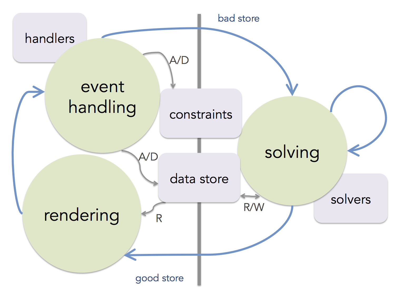
In order to support responsive interactive and animated programs, we adopt a two-phased execution model, cycling at an adjustable frame rate, e.g., 1/65 of a second. The clock time at the moment of each arrival on the first phase is used as the pseudo-time for the system. The two phases are: (A) event handling phase and (B) solving phase. The model is depicted in the figure below, which we'll explain next.

Two-phase execution model in CDP (A/D: add/delete, R/W: read/write)

(A) Event Handling Phase

The system starts in this phase, at top of which the system is considered to be at a "good" state and the current state is drawn on the canvas (should changes have occurred). The rendering step calls the draw methods for all objects to refresh the frame. At this time the system updates its pseudo-time to reflect the time passed since last cycle. The handlers for any cached events that may have occurred during the previous (B) phase are executed next. During such step the data and constraint stores may be modified. As a result, or despite of the fact, some constraints in the constraint store may have been unsatisfied. In any case, once all relevant handlers are executed, the system moves onto the phase B.

(B) Solving Phase

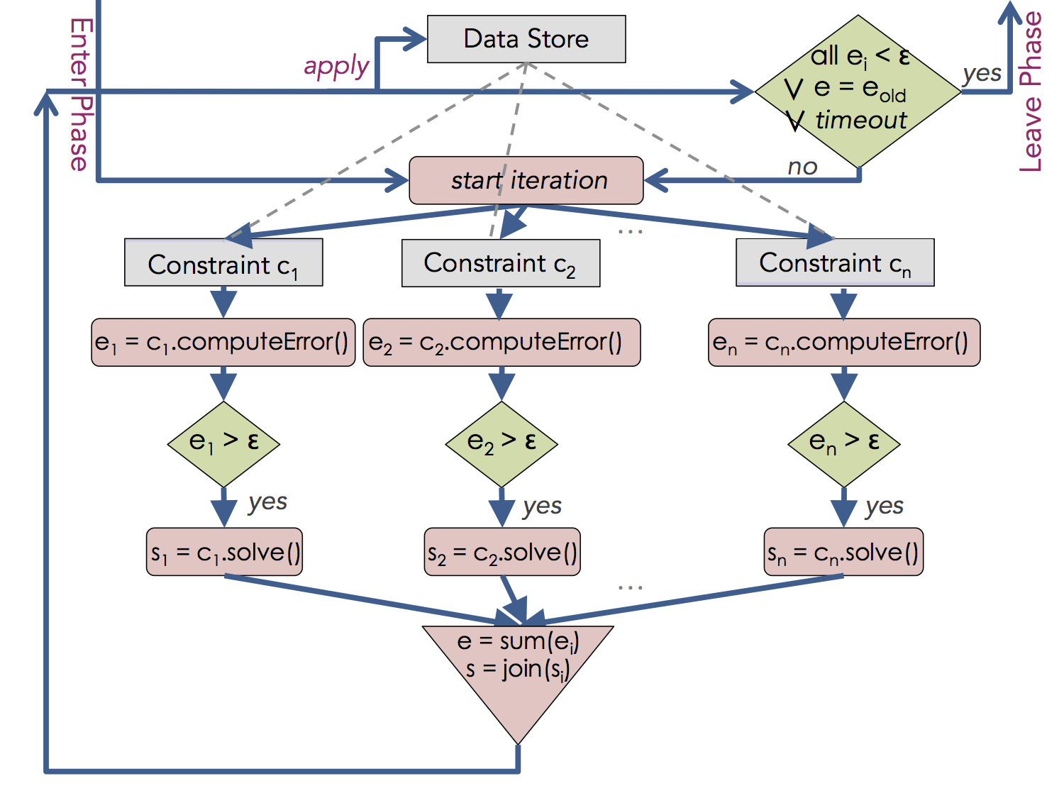
During the solving phase B (illustrated in figure below) the system invokes the computeError function belonging to each of the existing constraints. As long as the value is more than a an epsilon error threshold (specified by the user), the system invokes the solve function associated with each unsatisfied constraint. Each solution returned by each such function is organized as a dictionary of dictionaries, mapping each object's each property to a proposed value. Thus the value returned by a solve function could be interpreted as a patch: a subset of the current state that the constraint would like to change indicating the proposed new values.

At this point the system uses the designated merge function to combine all solutions to each variable into one consolidated new value, and then applies it to the variable. However, since these values aren't exactly what each constraint had asked for, after this step all or some of the previously unhappy constraints are likely to remain unhappy (or even previously happy constraints may have now turned unhappy). This is were the iterative relaxation approach comes in. As long as that is the case, the system repeats the process above, until either:

• (1) no unsatisfied constraints (computed error of larger than epsilon) remain.
• (2) the sum total error from all constraints remains unchanged for several consecutive iterations (reached a fixed-point).
• (3) phase B times out, that is, the system has remained in the solving phase for longer than the frame rate value.

At that point, the model cycles back to the reactive phase A, and this process repeats.

Solving phase

Classical backtracking search isn't accommodated by the CDP model as described. However, we have made a modification that allows programmers to rely on search as part of a program (see the pentominoes and send money demos).

We let a constraint type to be marked as searchable. A searchable constraint's solve function returns a set of solutions rather than one. Thus a user can communicate to the system that it wants to try either one of the solutions and search for the right combination of solutions from all constraints that will result in a globally acceptable solution.

During the first iteration of the solving phase (B), the system collects the set of solutions from each searchable constraint, as well as the usual one solution from others. It then constructs a search tree that gives all possible combinations of choosing a single solution from each constraint. (When no searchable constraint exists this tree has a single branch as the only combination to explore.) At this point the system engages in a traditional backtracking search to find the combination that leads to a satisfiable place. For each combination choice, it does the usual relaxing-style iterative solving up to some timeout duration, except that searchable constraints do not participate during those iterations. Should a fixed-point be reached with all constraints satisfied, the solution is committed and the model cycles back to the reactive phase A. Otherwise, solutions in the last attempt are discarded and the search of all possible combinations continues on.

As a simple example, below we have defined a NumListSortConstraint that ensures a number list is sorted. Provided that a copy of the list is kept in scratch.oldList, the computeError function returns a 0 error only when list has been properly sorted. The solve function simply returns all possible permutations of the list, therefore hinting to the system to search for one that would make the constraint satisfied.

NumListSortConstraint.prototype.searchable = true

NumListSortConstraint.prototype.computeError = function(pseudoTime) {
    return sorted(this.list)
        && isPermutationOf(this.list, scratch.oldList) ? 0 : 1
}

NumListSortConstraint.prototype.solve = function(pseudoTime) {
    return allPermutations(this.list).map(function (l) { return {list: l} })
}

Note that the above scheme works well when the numeric constraints solved by relaxation and finite domain constraints solved by search are mixed together within the same program, provided that numeric constraints use searched-over values in a read-only manner. Roughly speaking, if the relaxation-style iterative approach is like hill-climbing in some neighborhood in the state space, our augmented search-model is akin to simultaneously running hill-climbing in different regions in space in order to have a better chance of finding a solution. We're unclear as to whether the mixing makes sense if both kinds of constraints are trying to affect the same variables.